Follow one particle, then follow a crest. If those appear to make the same journey, the learner is confusing the motion of the medium with the motion of a wave. That distinction is a better starting point for a mechanics lesson than copying the wavelength formula alone.
Use the simple harmonic motion and mechanical-wave simulator as the main investigation, then connect it to force and work through the lever, friction, incline and pulley labs. This guide is based on the public wave-lab documentation reviewed on 18 November 2026 (Asia/Shanghai). The right-going wave case was measured in Light appearance on 18 November 2026 (Asia/Shanghai). A 30° lever preset and an n=3 pulley case were also logged as read-only checks. Parameter-change, incline and free-body readouts were not recorded and stay model predictions.
Investigation 1: local oscillation, traveling pattern
Set the wave controls explicitly:
| Control | Demonstration setting |
|---|---|
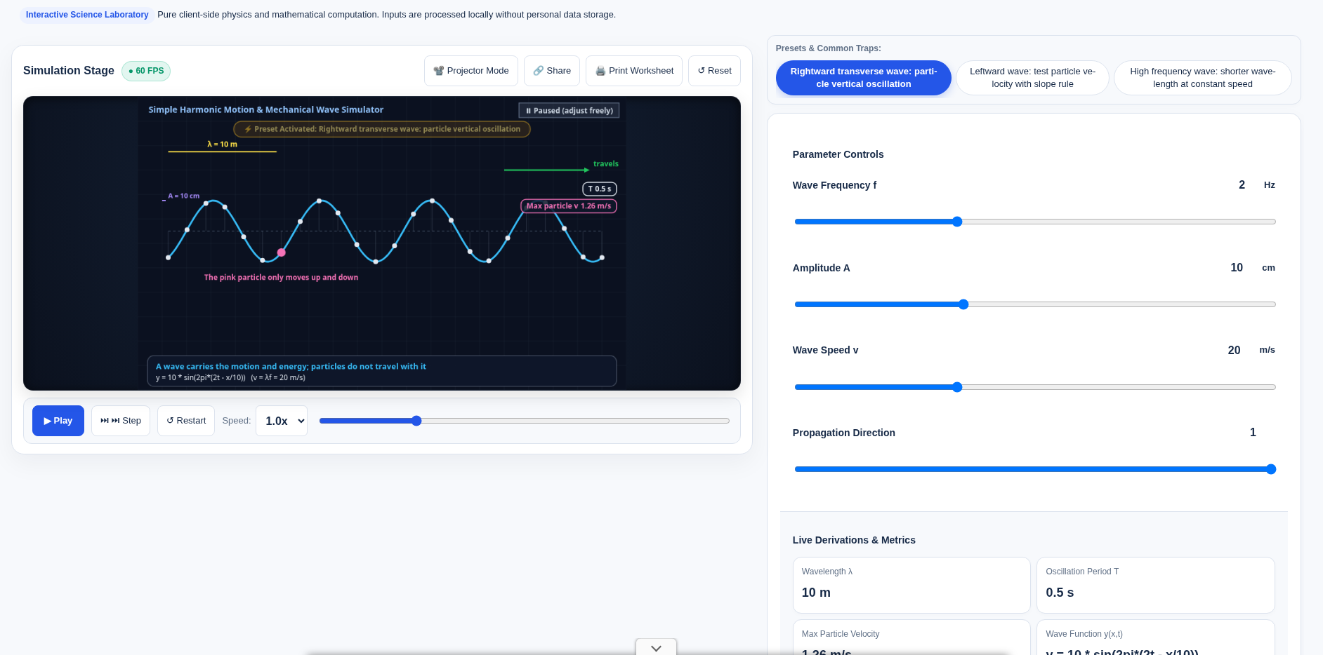
| Frequency f | 2.0 Hz |
| Amplitude A | 10 cm |
| Wave speed v | 20 m/s |
| Direction | Right-going |
| Animation speed | 1.0× |
The right-going transverse-wave preset is a convenient starting point; check its resulting controls before recording. The units above were checked in the public control markup, not inferred from an animation scale.
- Pick one identifiable particle at a fixed horizontal location. Predict its path before playing.
- Follow that particle through an oscillation, then pause. Does it migrate to the next particle’s location, or move about its own equilibrium?
- Follow a crest instead. Record which way the pattern moves, separately from which way the chosen particle is moving at that instant.
- Read the period and wavelength displays and compare them with
T=1/fandλ=v/f. Record their units as well as their numbers.
Expected model behavior: particles oscillate locally while the transverse wave pattern travels. A particle’s up/down speed is not the horizontal propagation speed. This is the model of an ideal transverse mechanical wave, not a complete description of ocean currents, breaking waves or drift of floating objects. OpenStax’s traveling-wave chapter makes the distinction between wave properties and the motion of the medium and explicitly notes the limits of simple ocean-wave comparisons.
At 07:39:07 Asia/Shanghai on 18 November 2026 (English capture 07:39:39), Reset was followed by the right-going transverse-wave preset and a pause. The controls were f=2 Hz, A=10 cm, wave speed v=20 m/s (metres per second, not centimetres per second), direction=1 (right), playback speed=1.0×. The display showed wavelength λ=10 m, period T=0.5 s, maximum particle velocity=1.26 m/s, and y = 10 * sin(2pi*(2t - x/10)). The page states v=λf, T=1/f and v_particle,max=ωA=2πfA. Converting A=10 cm to 0.10 m gives 2πfA≈1.26 m/s, matching the readout; do not multiply the centimetre amplitude into a metres-per-second speed. The preset text says the highlighted particle at x=5 m oscillates vertically in place rather than traveling with the wave. The English crop was cut above an overlapping ad, so the lower metric cards are clipped; λ, T, 1.26 m/s and the wave function remain visible on the wave itself.
Change one parameter and predict what should stay fixed
| Change | Hold fixed | Prediction for this controlled wave model |
|---|---|---|
| Increase frequency | Wave speed, amplitude | Period decreases; wavelength decreases |
| Increase amplitude | Frequency, wave speed | Larger displacement; same period and wavelength |
| Reverse propagation | Magnitudes of f, A and v | Pattern reverses; particles still oscillate locally |
If the readout gives maximum particle speed, compare its dependence on amplitude and frequency, not just wave speed. For a sinusoidal oscillation, v_particle,max=2πfA; convert amplitude from centimetres to metres when working in metres per second. The two speeds describe different motions.
A y–t graph follows one position over time. A y–x graph is many positions at one instant. Label those axes on paper before interpreting a slope. For a right-going profile y(x,t)=F(x−vt), local vertical velocity has the opposite sign to its spatial slope; for a left-going profile, the sign relation reverses. That rule assumes the stated traveling profile, not an arbitrary superposition of waves.
At an extreme displacement in ideal SHM, instantaneous speed is zero and acceleration points back toward equilibrium. At equilibrium crossing, speed is largest and displacement is zero. One frozen picture cannot by itself show the direction of motion; compare neighboring time steps or the documented propagation direction.
No before-and-after record was made for a frequency or amplitude change, or for a left-going wave, so the table below remains a model prediction rather than a second observed case. A dedicated y–t / y–x toggle is not assumed merely because the documentation discusses both graph types.
Investigation 2: a lever’s useful arm is perpendicular
Open the lever balance and moment-arm lab. Keep the load and the point where effort is applied fixed. Compare the perpendicular-force preset with the documented tilted-force setup at 30°.
Before comparing forces, draw the line of action and its perpendicular distance from the pivot. The distance along the bar is not automatically the moment arm:
L1 = d × sin θ
F1 × L1 = F2 × L2
Here θ is the angle between the effort direction and the bar-to-application-point direction in the model. A smaller effective arm requires a larger effort for the same balancing moment. The bar did not become shorter; the geometry changed. Ask students to explain the trend before reading the effort-force display.
In the lever lab, Reset was followed by the 30° tilted-effort preset: F2=100, L2=20 cm, d1=40 cm, θ=30°. The display showed F1=100 N, effective L1=20 cm, balancing moment=20 N·m, and a minimum force at 90° of 50 N. The substitution was F2×L2=100 N×0.2 m=20 N·m, L1=40 cm×sin30°=20 cm, F1=100 N, with the state labeled as an equal-arm lever. The 50 N figure is the minimum force shown for 90° in that same result, not a separately screenshotted perpendicular-force run.
Investigation 3: force reduction is not work reduction
Use two small comparisons rather than treating each machine as an unrelated formula.
Incline: in the inclined plane and screw-thread lab, compare the ideal smooth model with a frictional setting while keeping the height and load comparable. In a quasistatic, frictionless lift, F×L=G×h: a smaller effort requires a longer path. Friction adds input work. The wrapped-incline picture explains a screw’s geometric advantage; it does not specify a safe thread or fastening torque.
Pulley: in the block-and-tackle lab, count the rope sections actually supporting the movable assembly. Investigate the n=3 preset, then record effort and rope travel separately. In the ideal inextensible-rope geometry, s=n×h. With equal strand tension, negligible friction and movable-block weight included, the baseline is F=(G+G_movable)/n. Do not apply that baseline unchanged to a run with friction enabled. The page’s odd/even anchoring mnemonic describes its displayed classroom configurations, not every possible rigging arrangement or an instruction for lifting people.
For both, calculate useful work and input work under the same scenario. A force advantage is not free energy; ideal 100% efficiency means losses have been omitted. Real apparatus needs additional assumptions, and none of these animations is a rated lifting-system design.
Friction check: maximum is not the actual static force
The free-body and friction simulator is useful before claiming that any small push starts motion. Compare its documented 40 N and 60 N push presets, first checking mass, slope, coefficients and whether the block is initially at rest.
In the simple dry-friction model, static friction takes the value needed for equilibrium up to f_s,max=μ_s N; it is not always equal to that maximum. Once sliding, the model uses kinetic friction. On an incline, resolve the weight and normal force rather than using N=mg automatically. Do not infer precise real-material coefficients from this idealized transition.
The incline and free-body labs were not logged with numeric readouts and stay model descriptions. In the pulley lab, Reset was followed by the n=3 classroom-rigging preset: load G=300, movable-pulley weight=60, load-bearing strands n=3, lift height h=2, rope/friction loss f=10. The display showed rope-end force=130 N, rope travel=6 m, efficiency=76.92% and total work=780 J, with F=(300+60)/3+10=130 N and s=6 m. Useful work 300×2=600 J divided by 780 J matches that efficiency reading.
A short extension: projectile components are another representation problem
The projectile and trajectory lab can contrast horizontal motion with vertical acceleration. Keep it a classroom extension, not a range table. Equal launch/landing height, fixed initial speed, constant gravity and no drag are needed for the familiar 45° maximum-range statement; changing launch height changes that result. The animation is not a prediction of a real thrown object’s trajectory in wind.
Exit questions
- If frequency increases while wave speed is fixed, which changes: wavelength, amplitude or both? Explain the controlled variable.
- Why can tilting a force increase its required magnitude without moving the application point?
- Why does a pulley’s smaller effort not mean less input work?
Mark explanations of assumptions and mechanisms, not success at finding a preset. These are teaching models, not certified experiments or mechanical-safety approvals. The page’s local-processing wording is not an independent network audit. Keep a labeled particle-motion sketch and a separate force/work comparison as the lesson record.
Put this guide to work for your business
Start free tools with Google or an email code. Create a company and compare Pro plans when you need monitoring and team permissions.
Personal accounts use Free limits. A separate new company receives a 7-day Pro trial, excluding paid monthly credits.