A simulator becomes an experiment when students state what they will hold constant, predict a change and explain any disagreement. Start with double-slit fringe spacing, use the lens bench for a separate image-formation question, then move to an ideal-gas investigation with its own variables. Gas thermodynamics is not a branch of optics; the connection here is the method of controlled comparison.
The main activity uses the interference and diffraction simulator. This guide follows its public documentation reviewed on 18 November 2026 (Asia/Shanghai). Proposed trends are predictions from classroom models, not recorded live measurements unless explicitly identified as such.
Investigation 1: what sets double-slit fringe spacing?
Reset the lab, then explicitly select Red laser double-slit: 650nm wide fringes. Do not trust a highlighted preset without checking the parameter controls.
Record all four conditions:
| Quantity | What to record |
|---|---|
| Wavelength λ | Red preset: check the actual 650 nm setting |
| Slit separation d | Read the value in mm; do not confuse it with a single slit’s width |
| Screen distance L | Read the value in m |
| Experiment type | Double slit, type 1 |
Pause at a readable pattern and copy the live fringe-spacing value and substitution line, not the initial -- placeholder. Then make one controlled change at a time:
- Keep d and L fixed, shorten the wavelength and predict whether adjacent bright fringes become closer.
- Restore the starting wavelength, increase L and predict the spacing change.
- Restore L, increase d and predict the opposite trend.
- Explain the result with the same equation after each change, rather than citing the color alone.
For coherent double-slit interference at small angles and a sufficiently distant screen:
Δx ≈ Lλ/d
Use consistent units: nm and mm must be converted before mixing with metres. A convenient equivalent is Δx(mm)=L(m)×λ(nm)/(1000×d(mm)). This is dimensional conversion of the model, not a recorded result from the red preset.
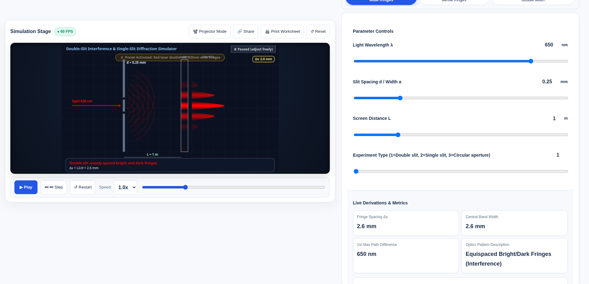
Recorded on 18 November 2026, 08:04 Asia/Shanghai, in the light theme: after Reset, the red 650 nm double-slit preset was clicked explicitly and the animation was paused. Experiment type was 1 (double slit), λ=650 nm, slit separation d=0.25 mm (the control is labelled “d / single-slit width a”), and screen distance L=1 m. Both the pattern and the metric cards showed fringe spacing Δx=2.6 mm, central band width w0=2.6 mm, first-maximum path difference 650 nm, and the pattern description “Equispaced Bright/Dark Fringes (Interference)”. The same live page displayed the substitution “L*lambda/d = 1m x 650nm / 0.25mm = 2.6mm”; that full line sits in the collapsed Live Derivations panel. This crop keeps the panel button and does not expand it. The dimensional check 1×650/(1000×0.25)=2.6 matches the live readout. The one-factor-at-a-time changes listed below were not recorded in this run and remain classroom predictions, not measured results.
OpenStax’s interference explanation derives the path-difference condition d sinθ=mλ and the small-angle screen approximation. It also notes intensity changes away from the center. Do not interpret a simplified equally spaced pattern as a promise that every real fringe has identical brightness.
Switch to single slit without carrying over the wrong meaning
In single-slit mode, the aperture parameter represents slit width a, not the distance between two slits. Predict the broad central maximum and weaker side structure. The far-field central width between the first minima is approximately 2Lλ/a; it is not the double-slit spacing with a new label. Keep the experiment type with every copied number.
This lab does not certify a real laser arrangement. Keep the activity virtual; a screen animation is not laser-safety guidance or a full account of every optical effect.
Investigation 2: locate a lens image before naming a device
Open the convex and concave lens bench. Reset and choose the documented Camera: u > 2f preset. Record focal length f, object distance u and object height in cm before reading image distance, magnification and image nature.
- Predict whether the converging lens gives a real or virtual image, and whether it is inverted or upright.
- Compare the ray intersections with the displayed image location.
- Keep f fixed and move the object into the range
f<u<2f, then inside the focal length. Predict the change before reading the labels. - If using the half-lens occlusion preset, ask whether fewer rays must mean half the object disappears.
For the ideal thin lens, take f>0 for a converging lens, u>0 for a real object, and v>0 for a real image (v<0 for a virtual image):
1/f = 1/u + 1/v
signed magnification m = −v/u
Report image orientation separately from the simulator’s displayed M: do not assume its M field uses the same signed convention. A real image forms where rays converge and can be intercepted by a screen; a virtual image is located by backward ray extensions. OpenStax’s thin-lens treatment provides the geometry and sign conventions.
The model predicts a complete but dimmer image when part of the aperture is blocked, not a simple missing half-picture. Actual illumination depends on the optical arrangement; do not claim an exact brightness fraction without a model that supports it. Thin-lens rays also omit real aberrations and finite-thickness details.
A supplemental check was made on the Chinese public page only; no extra screenshot was kept. After Reset, the camera preset labelled “【照相机原理】u > 2f 倒立缩小实像” was selected explicitly. The readouts were f=10 cm, u=25 cm, object height h0=5 cm; image distance v=16.67 cm; the magnification card showed M=−0.667× while the substitution line wrote m=−0.67x; image height h'=3.33 cm; the image was real, inverted and diminished, and the corresponding instrument was a camera. The half-occlusion preset was not recorded in this run.
Investigation 3: ideal gas—choose the held quantity, not just a law name
Use the separate ideal-gas law and p–V lab. Here p is pressure and V is volume; this is not a financial present-value calculator.
Reset and select the Boyle isothermal-compression preset. Record initial p in kPa, V in L and T in K, the process identifier and the actual endpoint state. For a fixed quantity of ideal gas, predict the pressure trend as volume decreases while temperature remains constant.
| Process | Held fixed | Relationship for fixed gas amount |
|---|---|---|
| Isothermal | T | pV is constant |
| Isochoric | V | p/T is constant |
| Isobaric | p | V/T is constant |
Use absolute temperature in kelvin and absolute pressure, not Celsius ratios or gauge pressure without conversion. The state relation is pV=nRT; it does not make a rapid real compression isothermal automatically.
A naming caution is essential here: the English tool calls its constant-volume preset “Isochoric heating (Charles)”; the Chinese isobaric preset uses “盖-吕萨克”. Record those as the tool’s labels, but identify the physical process by the held variable and the table above. Do not silently transfer a label to a different constraint.
Work signs need a declared convention
The tool has nR, W, ΔU and Q readouts. Copy their labels and values before comparing them. Its explanatory FAQ uses positive work on the gas. Another common convention, used in OpenStax’s first-law discussion, takes W_by positive for work by the gas:
ΔU = Q − W_by = Q + W_on
Do not switch conventions halfway through checking the balance. In an ideal-gas isothermal process, ΔU is zero; heat and work need not be zero. A p–V loop’s signed work also depends on traversal direction. The article does not assume the live W card’s convention merely from its English name.
This supplemental check was also made on the Chinese public page only, with no extra screenshot. On load, the Boyle preset chip appeared pressed while V1 read 2 L, even though the chip describes 4 L→2 L. After Reset and an explicit click on “【等温压缩:玻意耳定律】T不变,体积减半压强加倍”, V1 was 4 L. Inputs were p1=100 kPa, V1=4 L, T1=300 K, process id=1 (isothermal compression to V/2). The metric cards showed nR=1.33 J/K, W=−277.26 J, ΔU=0 J and Q=−277.26 J. The substitution line gave the final state p=200 kPa, V=2 L, T=300 K and wrote W and Q as −277.3 J. The card and substitution use different displayed precision; both are recorded as shown, without smoothing. The page itself distinguishes this gas p–V lab from the finance present-value tool.
Short extension: Doppler is a frequency question
The Doppler lab is useful for contrasting emitted frequency with wavefront arrival rate. Predict higher received pitch on approach and lower on recession in its acoustic setup, then record source, observer and medium-speed assumptions. A supplemental check on the Chinese public page, with no extra screenshot, used Reset and the ambulance preset: vs=30, f0=500 Hz, v=340, v0=0. The metric cards showed approaching 548.39 Hz, receding 459.46 Hz and Mach 0.0882 M; the preset chip was rounded to 548 Hz / 459 Hz. Both are recorded as displayed. Preset button frequencies are not measured readouts. Do not apply a sound-in-a-medium formula unchanged to relativistic light or cosmological redshift.
End by asking each learner to name one controlled variable, one observed trend and one model limitation. Correct algebra without those statements is not yet a complete experiment record. These labs are teaching models, not accredited curricula or safety approvals; local-processing wording is a page statement, not a network audit.
Put this guide to work for your business
Start free tools with Google or an email code. Create a company and compare Pro plans when you need monitoring and team permissions.
Personal accounts use Free limits. A separate new company receives a 7-day Pro trial, excluding paid monthly credits.